Chapter 15

— TWO —

A Brief Visit to the Systems Zoo

_____________

The . . . goal of all theory is to make the . . . basic elements as simple and as few as possible without having to surrender the adequate representation of . . . experience.

—Albert Einstein, ¹ physicist

One good way to learn something new is through specific examples rather than abstractions and generalities, so here are several common, simple but important examples of systems that are useful to understand in their own right and that will illustrate many general principles of complex systems.

This collection has some of the same strengths and weaknesses as a zoo. ² It gives you an idea of the large variety of systems that exist in the world, but it is far from a complete representation of that variety. It groups the animals by family—monkeys here, bears there (single-stock systems here, two-stock systems there)—so you can observe the characteristic behaviors of monkeys, as opposed to bears. But, like a zoo, this collection is too neat. To make the animals visible and understandable, it separates them from each other and from their normal concealing environment. Just as zoo animals more naturally occur mixed together in ecosystems, so the systems animals described here normally connect and interact with each other and with others not illustrated here—all making up the buzzing, hooting, chirping, changing complexity in which we live.

Ecosystems come later. For the moment, let’s look at one system animal at a time.

One-Stock Systems

A Stock with Two Competing Balancing Loops—a Thermostat

You already have seen the “homing in” behavior of the goal-seeking balancing feedback loop—the coffee cup cooling. What happens if there are two such loops, trying to drag a single stock toward two different goals?

One example of such a system is the thermostat mechanism that regulates the heating of your room (or cooling, if it is connected to an air conditioner instead of a furnace). Like all models, the representation of a thermostat in Figure 15 is a simplification of a real home heating system.

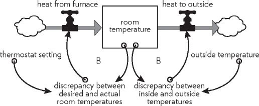
Figure 15. Room temperature regulated by a thermostat and furnace.

Whenever the room temperature falls below the thermostat setting, the thermostat detects a discrepancy and sends a signal that turns on the heat flow from the furnace, warming the room. When the room temperature rises again, the thermostat turns off the heat flow. This straightforward, stock-maintaining, balancing feedback loop is shown on the left side of Figure 15. If there were nothing else in the system, and if you start with a cold room with the thermostat set at 18°C (65°F), it would behave as shown in Figure 16. The furnace comes on, and the room warms up. When the room temperature reaches the thermostat setting, the furnace goes off, and the room stays right at the target temperature.

However, this is not the only loop in the system. Heat also leaks to the outside. The outflow of heat is governed by the second balancing feedback loop, shown on the right side of Figure 15. It is always trying to make the room temperature equal to the outside, just like a coffee cup cooling. If this were the only loop in the system (if there were no furnace), Figure 17 shows what would happen, starting with a warm room on a cold day.

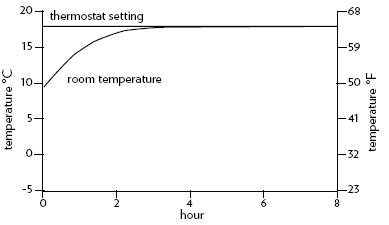
Figure 16. A cold room warms quickly to the thermostat setting.

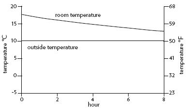
Figure 17. A warm room cools very slowly to the outside temperature of 10°C.

The assumption is that room insulation is not perfect, and so some heat leaks out of the warm room to the cool outdoors. The better the insulation, the slower the drop in temperature would be.

Now, what happens when these two loops operate at the same time? Assuming that there is sufficient insulation and a properly sized furnace, the heating loop dominates the cooling loop. You end up with a warm room (see Figure 18 ), even starting with a cold room on a cold day.

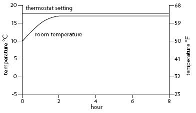
Figure 18. The furnace warms a cool room, even as heat continues to leak from the room.

As the room heats up, the heat flowing out of it increases, because there’s a larger gap between inside and outside temperatures. But the furnace keeps putting in more heat than the amount that leaks out, so the room warms nearly to the target temperature. At that point, the furnace cycles off and on as it compensates for the heat constantly flowing out of the room.

The thermostat is set at 18°C (65°F) in this simulation, but the room temperature levels off slightly below 18°C (65°F). That’s because of the leak to the outside, which is draining away some heat even as the furnace is getting the signal to put it back. This is a characteristic and sometimes surprising behavior of a system with competing balancing loops. It’s like trying to keep a bucket full when there’s a hole in the bottom. To make things worse, water leaking out of the hole is governed by a feedback loop; the more water in the bucket, the more the water pressure at the hole increases, so the flow out increases! In this case, we are trying to keep the room warmer than the outside and the warmer the room is, the faster it loses heat to the outside. It takes time for the furnace to correct for the increased heat loss—and in that minute still more heat leaks out. In a well-insulated house, the leak will be slower and so the house more comfortable than a poorly insulated one, even a poorly insulated house with a big furnace.

With home heating systems, people have learned to set the thermostat slightly higher than the actual temperature they are aiming at. Exactly how much higher can be a tricky question, because the outflow rate is higher on cold days than on warm days. But for thermostats this control problem isn’t serious. You can muddle your way to a thermostat setting you can live with.

For other systems with this same structure of competing balancing loops, the fact that the stock goes on changing while you’re trying to control it can create real problems. For example, suppose you’re trying to maintain a store inventory at a certain level. You can’t instantly order new stock to make up an immediately apparent shortfall. If you don’t account for the goods that will be sold while you are waiting for the order to come in, your inventory will never be quite high enough. You can be fooled in the same way if you’re trying to maintain a cash balance at a certain level, or the level of water in a reservoir, or the concentration of a chemical in a continuously flowing reaction system.

There’s an important general principle here, and also one specific to the thermostat structure. First the general one: The information delivered by a feedback loop can only affect future behavior; it can’t deliver the information, and so can’t have an impact fast enough to correct behavior that drove the current feedback. A person in the system who makes a decision based on the feedback can’t change the behavior of the system that drove the current feedback; the decisions he or she makes will affect only future behavior.

The information delivered by a feedback loop—even nonphysical feedback—can only affect future behavior; it can’t deliver a signal fast enough to correct behavior that drove the current feedback. Even nonphysical information takes time to feedback into the system.

Why is that important? Because it means there will always be delays in responding. It says that a flow can’t react instantly to a flow. It can react only to a change in a stock, and only after a slight delay to register the incoming information. In the bathtub, it takes a split second of time to assess the depth of the water and decide to adjust the flows. Many economic models make a mistake in this matter by assuming that consumption or production can respond immediately, say, to a change in price. That’s one of the reasons why real economies tend not to behave exactly like many economic models.

The specific principle you can deduce from this simple system is that you must remember in thermostat-like systems to take into account whatever draining or filling processes are going on. If you don’t, you won’t achieve the target level of your stock. If you want your room temperature to be at 18°C (65°F), you have to set the thermostat a little above the desired temperature. If you want to pay off your credit card (or the national debt), you have to raise your repayment rate high enough to cover the charges you incur while you’re paying (including interest). If you’re gearing up your work force to a higher level, you have to hire fast enough to correct for those who quit while you are hiring. In other words, your mental model of the system needs to include all the important flows, or you will be surprised by the system’s behavior.

A stock-maintaining balancing feedback loop must have its goal set appropriately to compensate for draining or inflowing processes that affect that stock. Otherwise, the feedback process will fall short of or exceed the target for the stock.

Before we leave the thermostat, we should see how it behaves with a varying outside temperature. Figure 19 shows a twenty-four-hour period of normal operation of a well-functioning thermostat system, with the outside temperature dipping well below freezing. The inflow of heat from the furnace nicely tracks the outflow of heat to the outside. The temperature in the room varies hardly at all once the room has warmed up.

Every balancing feedback loop has its breakdown point, where other loops pull the stock away from its goal more strongly than it can pull back. That can happen in this simulated thermostat system, if I weaken the power of the heating loop (a smaller furnace that cannot put out as much heat), or if I strengthen the power of the cooling loop (colder outside temperature, less insulation, or larger leaks). Figure 20 shows what happens with the same outside temperatures as in Figure 19, but with faster heat loss from the room. At very cold temperatures, the furnace just can’t keep up with the heat drain. The loop that is trying to bring the room temperature down to the outside temperature dominates the system for a while. The room gets pretty uncomfortable!

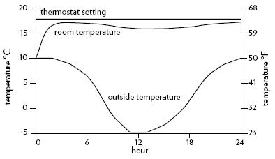
Figure 19. The furnace warms a cool room, even as heat leaks from the room and outside temperatures drop below freezing.

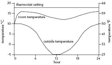
Figure 20. On a cold day, the furnace can’t keep the room warm in this leaky house!

See if you can follow, as time unfolds, how the variables in Figure 20 relate to one another. At first, both the room and the outside temperatures are cool. The inflow of heat from the furnace exceeds the leak to the outside, and the room warms up. For an hour or two, the outside is mild enough that the furnace replaces most of the heat that’s lost to the outside, and the room temperature stays near the desired temperature.

But as the outside temperature falls and the heat leak increases, the furnace cannot replace the heat fast enough. Because the furnace is generating less heat than is leaking out, the room temperature falls. Finally, the outside temperature rises again, the heat leak slows, and the furnace, still operating at full tilt, finally can pull ahead and start to warm the room again.

Just as in the rules for the bathtub, whenever the furnace is putting in more heat than is leaking out, the room temperature rises. Whenever the inflow rate falls behind the outflow rate, the temperature falls. If you study the system changes on this graph for a while and relate them to the feedback-loop diagram of this system, you’ll get a good sense of how the structural interconnections of this system—its two feedback loops and how they shift in strength relative to each other—lead to the unfolding of the system’s behavior over time.

A Stock with One Reinforcing Loop and One Balancing Loop—Population and Industrial Economy

What happens when a reinforcing and a balancing loop are both pulling on the same stock? This is one of the most common and important system structures. Among other things, it describes every living population and every economy.

A population has a reinforcing loop causing it to grow through its birth rate, and a balancing loop causing it to die off through its death rate.

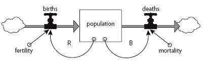
Figure 21. Population governed by a reinforcing loop of births and a balancing loop of deaths.

As long as fertility and mortality are constant (which in real systems they rarely are), this system has a simple behavior. It grows exponentially or dies off, depending on whether its reinforcing feedback loop determining births is stronger than its balancing feedback loop determining deaths.

For example, the 2007 world population of 6.6 billion people had a fertility rate of roughly 21 births a year for every 1,000 people in the population.Its mortality rate was 9 deaths a year out of every 1,000 people. Fertility was higher than mortality, so the reinforcing loop dominated the system. If those fertility and mortality rates continue unchanged, a child born now will see the world population more than double by the time he or she reaches the age of 60, as shown in Figure 22.

If, because of a terrible disease, the mortality rate were higher, say at 30 deaths per 1,000, while the fertility rate remained at 21, then the death loop would dominate the system. More people would die each year than would be born, and the population would gradually decrease (Figure 23).

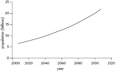
Figure 22. Population growth if fertility and mortality maintain their 2007 levels of 21 births and nine deaths per 1,000 people.

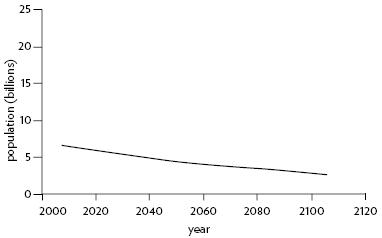
Figure 23. Population decline if fertility remains at 2007 level (21 births per 1,000) but mortality is much higher, 30 deaths per 1,000.

Things get more interesting when fertility and mortality change over time. When the United Nations makes long-range population projections, it generally assumes that, as countries become more developed, average fertility will decline (approaching replacement where on average each woman has 1.85 children). Until recently, assumptions about mortality were that it would also decline, but more slowly (because it is already low in most parts of the world). However, because of the epidemic of HIV/ AIDS, the UN now assumes the trend of increasing life expectancy over the next fifty years will slow in regions affected by HIV/AIDS.

Changing flows (fertility and mortality) create a change in the behavior over time of the stock (population)—the line bends. If, for example, world fertility falls steadily to equal mortality by the year 2035 and they both stay constant thereafter, the population will level off, births exactly balancing deaths in dynamic equilibrium, as in Figure 24.

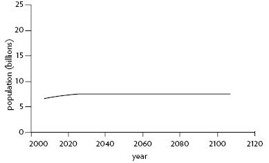
Figure 24. Population stabilizes when fertility equals mortality.

This behavior is an example of shifting dominance of feedback loops. Dominance is an important concept in systems thinking. When one loop dominates another, it has a stronger impact on behavior. Because systems often have several competing feedback loops operating simultaneously, those loops that dominate the system will determine the behavior.

At first, when fertility is higher than mortality, the reinforcing growth loop dominates the system and the resulting behavior is exponential growth. But that loop is gradually weakened as fertility falls. Finally, it exactly equals the strength of the balancing loop of mortality. At that point neither loop dominates, and we have dynamic equilibrium.

You saw shifting dominance in the thermostat system, when the outside temperature fell and the heat leaking out of the poorly insulated house overwhelmed the ability of the furnace to put heat into the room. Dominance shifted from the heating loop to the cooling loop.

Complex behaviors of systems often arise as the relative strengths of feedback loops shift, causing first one loop and then another to dominate behavior.

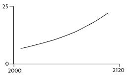
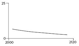
There are only a few ways a population system could behave, and these depend on what happens to the “driving” variables, fertility and mortality. These are the only ones possible for a simple system of one reinforcing and one balancing loop. A stock governed by linked reinforcing and balancing loops will grow exponentially if the reinforcing loop dominates the balancing one. It will die off if the balancing loop dominates the reinforcing one. It will level off if the two loops are of equal strength (see Figure 25 ). Or it will do a sequence of these things, one after another, if the relative strengths of the two loops change over time (see Figure 26 ).

I chose some provocative population scenarios here to illustrate a point about models and the scenarios they can generate. Whenever you are confronted with a scenario (and you are, every time you hear about an economic prediction, a corporate budget, a weather forecast, future climate change, a stockbroker saying what is going to happen to a particular holding), there are questions you need to ask that will help you decide how good a representation of reality is the underlying model.

• Are the driving factors likely to unfold this way? (What are birth rate and death rate likely to do?)

• If they did, would the system react this way? (Do birth and death rates really cause the population stock to behave as we think it will?)

• What is driving the driving factors? (What affects birth rate? What affects death rate?)

The first question can’t be answered factually. It’s a guess about the future, and the future is inherently uncertain. Although you may have a strong opinion about it, there’s no way to prove you’re right until the future actually happens. A systems analysis can test a number of scenarios to see what happens if the driving factors do different things. That’s usually one purpose of a systems analysis. But you have to be the judge of which scenario, if any, should be taken seriously as a future that might really be possible.

A: Growth

B: Decline

C: Stabilization

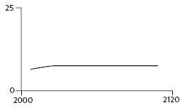
Figure 25. Three possible behaviors of a population: growth, decline, and stabilization.

Dynamic systems studies usually are not designed to predict what will happen. Rather, they’re designed to explore what would happen , if a number of driving factors unfold in a range of different ways.

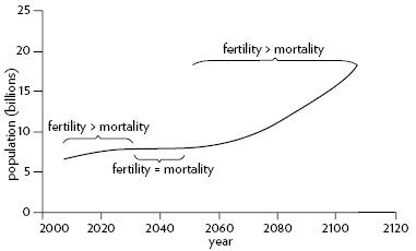
Figure 26. Shifting dominance of fertility and mortality loops.

The second question—whether the system really will react this way—is more scientific. It’s a question about how good the model is. Does it capture the inherent dynamics of the system? Regardless of whether you think the driving factors will do that, would the system behave like that if they did?

In the population scenarios above, however likely you think they are, the answer to this second question is roughly yes, the population would behave like this, if the fertility and mortality did that. The population model I have used here is very simple. A more detailed model would distinguish age groups, for example. But basically this model responds the way a real population would, growing under the conditions when a real population would grow, declining when a real population would decline. The numbers are off, but the basic behavior pattern is realistic.

System dynamics models explore possible futures and ask “what if” questions.

Finally, there is the third question. What is driving the driving factors?

QUESTIONS FOR TESTING THE VALUE OF A MODEL

1. Are the driving factors likely to unfold this way?

2. If they did, would the system react this way?

3. What is driving the driving factors?

Model utility depends not on whether its driving scenarios are realistic (since no one can know that for sure), but on whether it responds with a realistic pattern of behavior.

What is adjusting the inflows and outflows? This is a question about system boundaries. It requires a hard look at those driving factors to see if they are actually independent, or if they are also embedded in the system.

Is there anything about the size of the population, for instance, that might feed back to influence fertility or mortality? Do other factors—economics, the environment, social trends—influence fertility and mortality? Does the size of the population affect those economic and environmental and social factors?

Of course, the answer to all of these questions is yes. Fertility and mortality are governed by feedback loops too. At least some of those feedback loops are themselves affected by the size of the population. This population “animal” is only one piece of a much larger system. ³ Jay W. Forrester,

One important piece of the larger system that affects population is the economy. At the heart of the economy is another reinforcing-loop-plus-balancing- loop system—the same kind of structure, with the same kinds of behavior, as the population (see Figure 27 ).

The greater the stock of physical capital (machines and factories) in the economy and the efficiency of production (output per unit of capital), the more output (goods and services) can be produced each year.

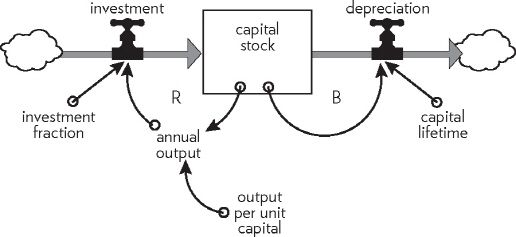
Figure 27. Like a living population, economic capital has a reinforcing loop (investment of output) governing growth and a balancing loop (depreciation) governing decline.

The more output that is produced, the more can be invested to make new capital. This is a reinforcing loop, like the birth loop for a population. The investment fraction is equivalent to the fertility. The greater the fraction of its output a society invests, the faster its capital stock will grow.

Physical capital is drained by depreciation—obsolescence and wearing out. The balancing loop controlling depreciation is equivalent to the death loop in a population. The “mortality” of capital is determined by the average capital lifetime. The longer the lifetime, the smaller the fraction of capital that must be retired and replaced each year.

If this system has the same structure as the population system, it must have the same repertoire of behaviors. Over recent history world capital, like world population, has been dominated by its reinforcing loop and has been growing exponentially. Whether in the future it grows or stays constant or dies off depends on whether its reinforcing growth loop remains stronger than its balancing depreciation loop. That depends on

• the investment fraction—how much output the society invests rather than consumes,

• the efficiency of capital—how much capital it takes to produce a given amount of output, and

• the average capital lifetime.

If a constant fraction of output is reinvested in the capital stock and the efficiency of that capital (its ability to produce output) is also constant, the capital stock may decline, stay constant, or grow, depending on the lifetime of the capital. The lines in Figure 28 show systems with different average capital lifetimes. With a relatively short lifetime, the capital wears out faster than it is replaced. Reinvestment does not keep up with depreciation and the economy slowly declines. When depreciation just balances investment, the economy is in dynamic equilibrium. With a long lifetime, the capital stock grows exponentially. The longer the lifetime of capital, the faster it grows.

This is another example of a principle we’ve already encountered: You can make a stock grow by decreasing its outflow rate as well as by increasing its inflow rate!

Just as many factors influence the fertility and mortality of a population, so many factors influence the output ratio, investment fraction, and the lifetime of capital—interest rates, technology, tax policy, consumption habits, and prices, to name just a few. Population itself influences investment, both by contributing labor to output, and by increasing demands on consumption, thereby decreasing the investment fraction. Economic output also feeds back to influence population in many ways. A richer economy usually has better health care and a lower death rate. A richer economy also usually has a lower birth rate.

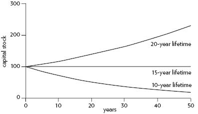
Figure 28. Growth in capital stock with changes in the lifetime of the capital. In a system with output per unit capital ratio of 1:3 and an investment fraction of 20 percent, capital with a lifetime of 15 years just keeps up with depreciation. A shorter lifetime leads to a declining stock of capital.

In fact, just about any long term model of a real economy should link together the two structures of population and capital to show how they affect each other. The central question of economic development is how to keep the reinforcing loop of capital accumulation from growing more slowly than the reinforcing loop of population growth—so that people are getting richer instead of poorer. ⁴

It may seem strange to you that I call the capital system the same kind of “zoo animal” as the population system. A production system with factories and shipments and economic flows doesn’t look much like a population system with babies being born and people aging and having more babies and dying. But from a systems point of view these systems, so dissimilar in many ways, have one important thing in common: their feedback-loop structures. Both have a stock governed by a reinforcing growth loop and a balancing death loop.Both also have an aging process. Steel mills and lathes and turbines get older and die just as people do.

Systems with similar feedback structures produce similar dynamic behaviors.

One of the central insights of systems theory, as central as the observation that systems largely cause their own behavior, is that systems with similar feedback structures produce similar dynamic behaviors, even if the outward appearance of these systems is completely dissimilar.

A population is nothing like an industrial economy, except that both can reproduce themselves out of themselves and thus grow exponentially. And both age and die. A coffee cup cooling is like a warmed room cooling, and like a radioactive substance decaying, and like a population or industrial economy aging and dying. Each declines as the result of a balancing feedback loop.

A System with Delays—Business Inventory

Picture a stock of inventory in a store—a car dealership—with an inflow of deliveries from factories and an outflow of new car sales. By itself, this stock of cars on the dealership lot would behave like the water in a bathtub.

Now picture a regulatory feedback system designed to keep the inventory high enough so that it can always cover ten days’ worth of sales (see Figure 29 ). The car dealer needs to keep some inventory because deliveries and purchases don’t match perfectly every day. Customers make purchases that are unpredictable on a day-to-day basis. The car dealer also needs to provide herself with some extra inventory (a buffer) in case deliveries from suppliers are delayed occasionally.

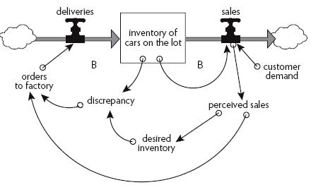
Figure 29. Inventory at a car dealership is kept steady by two competing balancing loops, one through sales and one through deliveries.

The dealer monitors sales (perceived sales), and if, for example, they seem to be rising, she adjusts orders to the factory to bring inventory up to her new desired inventory that provides ten days’ coverage at the higher sales rate. So, higher sales mean higher perceived sales, which means a higher discrepancy between inventory and desired inventory, which means higher orders, which will bring in more deliveries, which will raise inventory so it can comfortably supply the higher rate of sales.

This system is a version of the thermostat system—one balancing loop of sales draining the inventory stock and a competing balancing loop maintaining the inventory by resupplying what is lost in sales. Figure 30 shows the not very surprising result of an increase in consumer demand of 10 percent.

In Figure 31, I am putting something else into this simple model—three delays that are typical of what we experience in the real world.

First, there is a perception delay, intentional in this case. The car dealer doesn’t react to just any blip in sales. Before she makes ordering decisions, she averages sales over the past five days to sort out real trends from temporary dips and spikes.

Second, there is a response delay. Even when it’s clear that orders need to be adjusted, she doesn’t try to make up the whole adjustment in a single order. Rather, she makes up one-third of any shortfall with each order. Another way of saying that is, she makes partial adjustments over three days to be extra sure the trend is real. Third, there is a delivery delay. It takes five days for the supplier at the factory to receive an order, process it, and deliver it to the dealership.

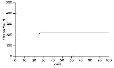
Figure 30. Inventory on the car dealership’s lot with a permanent 10-percent increase in consumer demand starting on day 25.

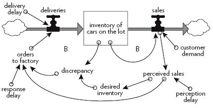
Figure 31. Inventory at a car dealership with three common delays now included in the picture—a perception delay, a response delay, and a delivery delay.

Although this system still consists of just two balancing loops, like the simplified thermostat system, it doesn’t behave like the thermostat system. Look at what happens, for example, as shown in Figure 32, when the business experiences the same permanent 10-percent jump in sales from an increase in customer demand.

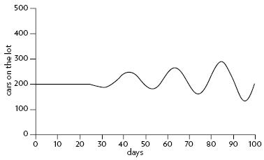
Figure 32. Response of inventory to a 10-percent increase in sales when there are delays in the system.

Oscillations! A single step up in sales causes inventory to drop. The car dealer watches long enough to be sure the higher sales rate is going to last. Then she begins to order more cars to both cover the new rate of sales and bring the inventory up. But it takes time for the orders to come in. During that time inventory drops further, so orders have to go up a little more, to bring inventory back up to ten days’ coverage.

Eventually, the larger volume of orders starts arriving, and inventory recovers—and more than recovers, because during the time of uncertainty about the actual trend, the owner has ordered too much. She now sees her mistake, and cuts back, but there are still high past orders coming in, so she orders even less. In fact, almost inevitably, since she still can’t be sure of what is going to happen next, she orders too little. Inventory gets too low again. And so forth, through a series of oscillations around the new desired inventory level. As Figure 33 illustrates, what a difference a few delays make!

We’ll see in a moment that there are ways to damp these oscillations in inventory, but first it’s important to understand why they occur. It isn’t because the car dealer is stupid. It’s because she is struggling to operate in a system in which she doesn’t have, and can’t have, timely information and in which physical delays prevent her actions from having an immediate effect on inventory. She doesn’t know what her customers will do next. When they do something, she’s not sure they’ll keep doing it. When she issues an order, she doesn’t see an immediate response. This situation of information insufficiency and physical delays is very common. Oscillations like these are frequently encountered in inventories and in many other systems. Try taking a shower sometime where there’s a very long pipe between the hot- and cold-water mixer and the showerhead, and you’ll experience directly the joys of hot and cold oscillations because of a long response delay.

A delay in a balancing feedback loop makes a system likely to oscillate.

How much of a delay causes what kind of oscillation under what circumstances is not a simple matter. I can use this inventory system to show you why.

“These oscillations are intolerable,” says the car dealer (who is herself a learning system, determined now to change the behavior of the inventory system). “I’m going to shorten the delays. There’s not much I can do about the delivery delay from the factory, so I’m going to react faster myself. I’ll average sales trends over only two days instead of five before I make order adjustments.”

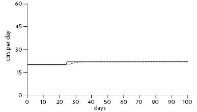
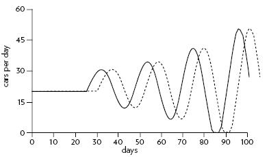
Figure 33. The response of orders and deliveries to an increase in demand. A shows the small but sharp step up in sales on day 25 and the car dealer’s “perceived” sales, in which she averages the change over 3 days. B shows the resulting ordering pattern, tracked by the actual deliveries from the factory.

Figure 34 illustrates what happens when the dealer’s perception delay is shortened from five days to two.

Not much happens when the car dealer shortens her perception delay. If anything the oscillations in the inventory of cars on the lot are a bit worse. And if, instead of shortening her perception time, the car dealer tries shortening her reaction time—making up perceived shortfalls in two days instead of three—things get very much worse, as shown in Figure 35.

Something has to change and, since this system has a learning person within it, something will change. “High leverage, wrong direction,” the system-thinking car dealer says to herself as she watches this failure of a policy intended to stabilize the oscillations. This perverse kind of result can be seen all the time—someone trying to fix a system is attracted intuitively to a policy lever that in fact does have a strong effect on the system. And then the well-intentioned fixer pulls the lever in the wrong direction! This is just one example of how we can be surprised by the counterintuitive behavior of systems when we start trying to change them.

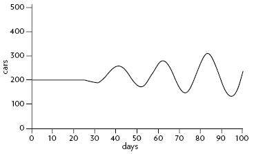
Figure 34. The response of inventory to the same increase in demand with a shortened perception delay.

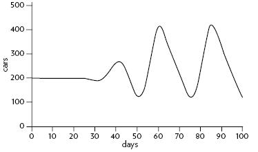
Figure 35. The response of inventory to the same increase in demand with a shortened reaction time. Acting faster makes the oscillations worse!

Part of the problem here is that the car dealer has been reacting not too slowly, but too quickly. Given the configuration of this system, she has been overreacting. Things would go better if, instead of decreasing her response delay from three days to two, she would increase the delay from three days to six, as illustrated in Figure 36.

As Figure 36 shows, the oscillations are greatly damped with this change, and the system finds its new equilibrium fairly efficiently.

Delays are pervasive in systems, and they are strong determinants of behavior. Changing the length of a delay may (or may not, depending on the type of delay and the relative lengths of other delays) make a large change in the behavior of a system.

The most important delay in this system is the one that is not under the direct control of the car dealer. It’s the delay in delivery from the factory. But even without the ability to change that part of her system, the dealer can learn to manage inventory quite well.

Changing the delays in a system can make it much easier or much harder to manage. You can see why system thinkers are somewhat fanatic on the subject of delays. We’re always on the alert to see where delays occur in systems, how long they are, whether they are delays in information streams or in physical processes. We can’t begin to understand the dynamic behavior of systems unless we know where and how long the delays are. And we are aware that some delays can be powerful policy levers. Lengthening or shortening them can produce major changes in the behavior of systems.

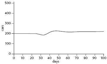
Figure 36. The response of inventory to the same increase in demand with a slowed reaction time.

In the big picture, one store’s inventory problem may seem trivial and fixable. But imagine that the inventory is that of all the unsold automobiles in America. Orders for more or fewer cars affect production not only at assembly plants and parts factories, but also at steel mills, rubber and glass plants, textile producers, and energy producers. Everywhere in this system are perception delays, production delays, delivery delays, and construction delays. Now consider the link between car production and jobs—increased production increases the number of jobs allowing more people to buy cars. That’s a reinforcing loop, which also works in the opposite direction—less production, fewer jobs, fewer car sales, less production. Put in another reinforcing loop, as speculators buy and sell shares in the auto and auto-supply companies based on their recent performance, so that an upsurge in production produces an upsurge in stock price, and vice versa.

That very large system, with interconnected industries responding to each other through delays, entraining each other in their oscillations, and being amplified by multipliers and speculators, is the primary cause of business cycles. Those cycles don’t come from presidents, although presidents can do much to ease or intensify the optimism of the upturns and the pain of the downturns. Economies are extremely complex systems; they are full of balancing feedback loops with delays, and they are inherently oscillatory. ⁵ Jay W. Forrester, 1989.

Two-Stock Systems

A Renewable Stock Constrained by a Nonrenewable Stock—an Oil Economy

The systems I’ve displayed so far have been free of constraints imposed by their surroundings. The capital stock of the industrial economy model didn’t require raw materials to produce output. The population didn’t need food. The thermostat-furnace system never ran out of oil. These simple models of the systems have been able to operate according to their unconstrained internal dynamics, so we could see what those dynamics are.

But any real physical entity is always surrounded by and exchanging things with its environment. A corporation needs a constant supply of energy and materials and workers and managers and customers. A growing corn crop needs water and nutrients and protection from pests. A population needs food and water and living space, and if it’s a human population, it needs jobs and education and health care and a multitude of other things. Any entity that is using energy and processing materials needs a place to put its wastes, or a process to carry its wastes away.

Therefore, any physical, growing system is going to run into some kind of constraint, sooner or later. That constraint will take the form of a balancing loop that in some way shifts the dominance of the reinforcing loop driving the growth behavior, either by strengthening the outflow or by weakening the inflow.

Growth in a constrained environment is very common, so common that systems thinkers call it the “limits-to-growth” archetype. (We’ll explore more archetypes—frequently found system structures that produce familiar behavior patterns—in Chapter Five.) Whenever we see a growing entity, whether it be a population, a corporation, a bank account, a rumor, an epidemic, or sales of a new product, we look for the reinforcing loops that are driving it and for the balancing loops that ultimately will constrain it. We know those balancing loops are there, even if they are not yet dominating the system’s behavior, because no real physical system can grow forever. Even a hot new product will saturate the market eventually. A chain reaction in a nuclear power plant or bomb will run out of fuel. A virus will run out of susceptible people to infect. An economy may be constrained by physical capital or monetary capital or labor or markets or management or resources or pollution.

In physical, exponentially growing systems, there must be at least one reinforcing loop driving the growth and at least one balancing loop constraining the growth, because no physical system can grow forever in a finite environment.

Like resources that supply the inflows to a stock, a pollution constraint can be renewable or nonrenewable. It’s nonrenewable if the environment has no capacity to absorb the pollutant or make it harmless. It’s renewable if the environment has a finite, usually variable, capacity for removal. Everything said here about resource-constrained systems, therefore, applies with the same dynamics but opposite flow directions to pollution-constrained systems.

The limits on a growing system may be temporary or permanent. The system may find ways to get around them for a short while or a long while, but eventually there must come some kind of accommodation, the system adjusting to the constraint, or the constraint to the system, or both to each other. In that accommodation come some interesting dynamics.

Whether the constraining balancing loops originate from a renewable or nonrenewable resource makes some difference, not in whether growth can continue forever, but in how growth is likely to end.

Let’s look, to start, at a capital system that makes its money by extracting a nonrenewable resource—say an oil company that has just discovered a huge new oil field. See Figure 37 .

The diagram in Figure 37 may look complicated, but it’s no more than a capital-growth system like the one we’ve already seen, using “profit” instead of “output.” Driving depreciation is the now-familiar balancing loop: the more capital stock, the more machines and refineries there are that fall apart and wear out, reducing the stock of capital. In this example, the capital stock of oil drilling and refining equipment depreciates with a 20-year lifetime—meaning 1/20 (or 5 percent) of the stock is taken out of commission each year. It builds itself up through investment of profits from oil extraction. So we see the reinforcing loop: More capital allows more resource extraction, creating more profits that can be reinvested. I’ve assumed that the company has a goal of 5 percent annual growth in its business capital. If there isn’t enough profit for 5 percent growth, the company invests whatever profits it can.

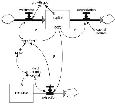
Figure 37. Economic capital, with its reinforcing growth loop constrained by a nonrenewable resource.

Profit is income minus cost. Income in this simple representation is just the price of oil times the amount of oil the company extracts. Cost is equal to capital times the operating cost (energy, labor, materials, etc.) per unit of capital. For the moment, I’ll make the simplifying assumptions that both price and operating cost per unit of capital are constant.

What is not assumed to be constant is the yield of resource per unit of capital. Because this resource is not renewable, as in the case of oil, the stock feeding the extraction flow does not have an input. As the resource is extracted—as an oil well is depleted—the next barrel of oil becomes harder to get. The remaining resource is deeper down, or more dilute, or in the case of oil, under less natural pressure to force it to the surface. More and more costly and technically sophisticated measures are required to keep the resource coming.

Here is a new balancing feedback loop that ultimately will control the growth of capital: the more capital, the higher the extraction rate. The higher the extraction rate, the lower the resource stock. The lower the resource stock, the lower the yield of resource per unit of capital, so the lower the profit (with price assumed constant) and the lower the investment rate—therefore, the lower the rate of growth of capital. I could assume that resource depletion feeds back through operating cost as well as capital efficiency. In the real world it does both. In either case, the ensuing behavior pattern is the same—the classic dynamics of depletion (see Figure 38 ).

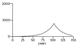
The system starts out with enough oil in the underground deposit to supply the initial scale of operation for 200 years. But, actual extraction peaks at about 40 years because of the surprising effect of exponential growth in extraction. At an investment rate of 10 percent per year, the capital stock and therefore the extraction rate both grow at 5 percent per year and so double in the first 14 years. After 28 years, while the capital stock has quadrupled, extraction is starting to lag because of falling yield per unit of capital. By year 50 the cost of maintaining the capital stock has overwhelmed the income from resource extraction, so profits are no longer sufficient to keep investment ahead of depreciation. The operation quickly shuts down, as the capital stock declines. The last and most expensive of the resource stays in the ground; it doesn’t pay to get it out.

A: Extraction rate

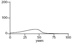
B: Capital stock

C: Resource stock

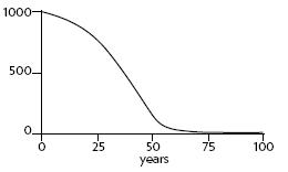
Figure 38. Extraction (A) creates profits that allow for growth of capital (B) while depleting the nonrenewable resource (C). The greater the accumulation of capital, the faster the resource is depleted.

What happens if the original resource turns out to be twice as large as the geologists first thought—or four times as large? Of course, that makes a huge difference in the total amount of oil that can be extracted from this field. But with the continued goal of 10 percent per year reinvestment producing 5 percent per year capital growth, each doubling of the resource makes a difference of only about 14 years in the timing of the peak extraction rate, and in the lifetime of any jobs or communities dependent on the extraction industry (see Figure 39 ).

A quantity growing exponentially toward a constraint or limit reaches that limit in a surprisingly short time.

The higher and faster you grow, the farther and faster you fall, when you’re building up a capital stock dependent on a nonrenewable resource. In the face of exponential growth of extraction or use, a doubling or quadrupling of the nonrenewable resource give little added time to develop alternatives.

If your concern is to extract the resource and make money at the maximum possible rate, then the ultimate size of the resource is the most important number in this system. If, say, you’re a worker at the mine or oil field, and your concern is with the lifetime of your job and stability of your community, then there are two important numbers: the size of the resource and the desired growth rate of capital. (Here is a good example of the goal of a feedback loop being crucial to the behavior of a system.) The real choice in the management of a nonrenewable resource is whether to get rich very fast or to get less rich but stay that way longer.

The graph in Figure 40 shows the development of the extraction rate over time, given desired growth rates above depreciation varying from 1 percent annually, to 3 percent, 5 percent, and 7 percent. With a 7 percent growth rate, extraction of this “200-year supply” peaks within 40 years. Imagine the effects of this choice not only on the profits of the company, but on the social and natural environments of the region.

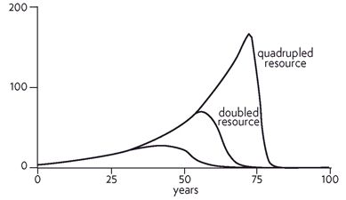
Figure 39. Extraction with two times or four times as large a resource to draw on. Each doubling of the resource makes a difference of only about fourteen years in the peak of extraction.

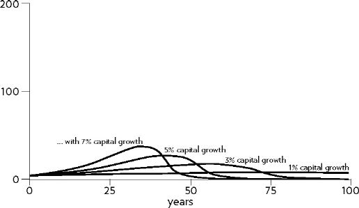
Figure 40. The peak of extraction comes much more quickly as the fraction of profits reinvested increases.

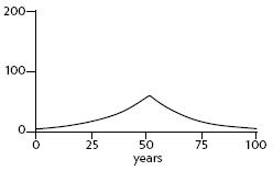
Earlier I said I would make the simplifying assumption that price was constant. But what if that’s not true? Suppose that in the short term the resource is so vital to consumers that a higher price won’t decrease demand. In that case, as the resource gets scarce and price rises steeply, as shown in Figure 41.

The higher price gives the industry higher profits, so investment goes up, capital stock continues rising, and the more costly remaining resources can be extracted. If you compare Figure 41 with Figure 38, where price was held constant, you can see that the main effect of rising price is to build the capital stock higher before it collapses.

The same behavior results, by the way, if prices don’t go up but if technology brings operating costs down—as has actually happened, for example, with advanced recovery techniques from oil wells, with the beneficiation process to extract low-grade taconite from exhausted iron mines, and with the cyanide leaching process that allows profitable extraction even from the tailings of gold and silver mines.

We all know that individual mines and fossil fuel deposits and groundwater aquifers can be depleted. There are abandoned mining towns and oil fields all over the world to testify to the reality of the behavior we’ve seen here. Resource companies understand this dynamic too. Well before depletion makes capital less efficient in one place, companies shift investment to discovery and development of another deposit somewhere else. But, if there are local limits, eventually will there be global ones?

A: Extraction rate

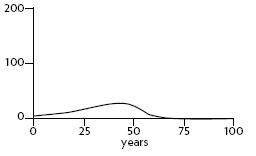
B: Capital stock

C: Resource stock

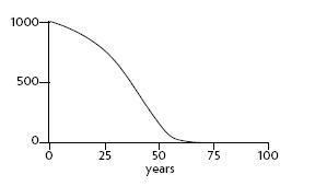
Figure 41. As price goes up with increasing scarcity, there is more profit to reinvest, and the capital stock can grow larger (B) driving extraction up for longer (A). The consequence is that the resource (C) is depleted even faster at the end.

I’ll leave you to have this argument with yourself, or with someone of the opposite persuasion. I will just point out that, according to the dynamics of depletion, the larger the stock of initial resources, the more new discoveries, the longer the growth loops elude the control loops, and the higher the capital stock and its extraction rate grow, and the earlier, faster, and farther will be the economic fall on the back side of the production peak.

Unless, perhaps, the economy can learn to operate entirely from renewable resources.

Renewable Stock Constrained by a Renewable Stock—a Fishing Economy

Assume the same capital system as before, except that now there is an inflow to the resource stock, making it renewable. The renewable resource in this system could be fish and the capital stock could be fishing boats. It also could be trees and sawmills, or pasture and cows. Living renewable resources such as fish or trees or grass can regenerate themselves from themselves with a reinforcing feedback loop. Nonliving renewable resources such as sunlight or wind or water in a river are regenerated not through a reinforcing loop, but through a steady input that keeps refilling the resource stock no matter what the current state of that stock might be. This same “renewable resource system” structure occurs in an epidemic of a cold virus. It spares its victims who are then able to catch another cold. Sales of a product people need to buy regularly is also a renewable resource system; the stock of potential customers is ever regenerated. Likewise an insect infestation that destroys part but not all of a plant; the plant can regenerate and the insect can eat more. In all these cases, there is an input that keeps refilling the constraining resource stock (as shown in Figure 42).

We will use the example of a fishery. Once again, assume that the lifetime of capital is 20 years and the industry will grow, if it can, at 5 percent per year. As with the nonrenewable resource, assume that as the resource gets scarce it costs more, in terms of capital, to harvest it. Bigger fishing boats that can go longer distances and are equipped with sonar are needed to find the last schools of fish. Or miles-long drift nets are needed to catch them. Or on-board refrigeration systems are needed to bring them back to port from longer distances. All this takes more capital.

The regeneration rate of the fish is not constant, but is dependent on the number of fish in the area—fish density. If the fish are very dense, their reproduction rate is near zero, limited by available food and habitat. If the fish population falls a bit, it can regenerate at a faster and faster rate, because it can take advantage of unused nutrients or space in the ecosystem. But at some point the fish reproduction rate reaches its maximum. If the population is further depleted, it breeds not faster and faster, but slower and slower. That’s because the fish can’t find each other, or because another species has moved into its niche.

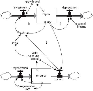
Figure 42. Economic capital with its reinforcing growth loop constrained by a renewable resource.

This simplified model of a fishery economy is affected by three nonlinear relationships: price (scarcer fish are more expensive); regeneration rate (scarcer fish don’t breed much, nor do crowded fish); and yield per unit of capital (efficiency of the fishing technology and practices).

This system can produce many different sets of behaviors. Figure 43 shows one of them.

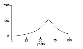
In Figure 43, we see capital and fish harvest rise exponentially at first. The fish population (the resource stock) falls, but that stimulates the fish reproduction rate. For decades the resource can go on supplying an exponentially increasing harvest rate. Eventually, the harvest rises too far and the fish population falls low enough to reduce the profitability of the fishing fleet. The balancing feedback of falling harvest reducing profits brings down the investment rate quickly enough to bring the fishing fleet into equilibrium with the fish resource. The fleet can’t grow forever, but it can maintain a high and steady harvest rate forever.

Just a minor change in the strength of the controlling balancing feedback loop through yield per unit of capital, however, can make a surprising difference. Suppose that in an attempt to raise the catch in the fishery, the industry comes up with a technology to improve the efficiency of the boats (sonar, for example, to find the scarcer fish). As the fish population declines, the fleet’s ability to pull in the same catch per boat is maintained just a little longer (see Figure 44 ).

A: Harvest rate

B: Capital stock

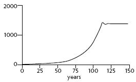
C: Resource stock

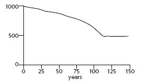
Figure 43. Annual harvest (A) creates profits that allow for growth of capital stock (B), but the harvest levels off, after a small overshoot in this case. The result of leveling harvest is that the resource stock (C) also stabilizes.

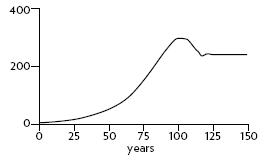
Figure 44 shows another case of high leverage, wrong direction! This technical change, which increases the productivity of all fishermen, throws the system into instability. Oscillations appear!

A: Harvest rate

B: Capital stock

C: Resource stock

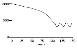
Figure 44. A slight increase in yield per unit of capital—increasingly efficient technology in this case—creates a pattern of overshoot and oscillation around a stable value in the harvest rate (A), the stock of economic capital (B), and in the resource stock.

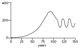
A: Harvest rate

B: Capital stock

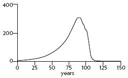
C: Resource stock

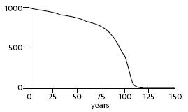
Figure 45. An even greater increase in yield per unit of capital creates a patterns of overshoot and collapse in the harvest (A), the economic capital (B), and the resource (C).

If the fishing technology gets even better, the boats can go on operating economically even at very low fish densities. The result can be a nearly complete wipeout both of the fish and of the fishing industry. The consequence is the marine equivalent of desertification. The fish have been turned, for all practical purposes, into a nonrenewable resource. Figure 45 illustrates this scenario.

Nonrenewable resources are stock -limited. The entire stock is available at once, and can be extracted at any rate (limited mainly by extraction capital). But since the stock is not renewed, the faster the extraction rate, the shorter the lifetime of the resource.

Renewable resources are flow limited. They can support extraction or harvest indefinitely, but only at a finite flow rate equal to their regeneration rate. If they are extracted faster than they regenerate, they may eventually be driven below a critical threshold and become, for all practical purposes, nonrenewable.

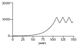
In many real economies based on real renewable resources—as opposed to this simple model—the very small surviving population retains the potential to build its numbers back up again, once the capital driving the harvest is gone. The whole pattern is repeated, decades later. Very long term renewable-resource cycles like these have been observed, for example, in the logging industry in New England, now in its third cycle of growth, overcutting, collapse, and eventual regeneration of the resource. But this is not true for all resource populations. More and more, increases in technology and harvest efficiency have the ability to drive resource populations to extinction.

Whether a real renewable resource system can survive overharvest depends on what happens to it during the time when the resource is severely depleted. A very small fish population may become especially vulnerable to pollution or storms or lack of genetic diversity. If this is a forest or grassland resource, the exposed soils may be vulnerable to erosion. Or the nearly empty ecological niche may be filled in by a competitor. Or perhaps the depleted resource can survive and rebuild itself again.

I’ve shown three sets of possible behaviors of this renewable resource system here:

• overshoot and adjustment to a sustainable equilibrium,

• overshoot beyond that equilibrium followed by oscillation around it, and

• overshoot followed by collapse of the resource and the industry dependent on the resource.

Which outcome actually occurs depends on two things. The first is the critical threshold beyond which the resource population’s ability to regenerate itself is damaged. The second is the rapidity and effectiveness of the balancing feedback loop that slows capital growth as the resource becomes depleted. If the feedback is fast enough to stop capital growth before the critical threshold is reached, the whole system comes smoothly into equilibrium. If the balancing feedback is slower and less effective, the system oscillates. If the balancing loop is very weak, so that capital can go on growing even as the resource is reduced below its threshold ability to regenerate itself, the resource and the industry both collapse.

Neither renewable nor nonrenewable limits to growth allow a physical stock to grow forever, but the constraints they impose are dynamically quite different. The difference comes because of the difference between stocks and flows.

The trick, as with all the behavioral possibilities of complex systems, is to recognize what structures contain which latent behaviors, and what conditions release those behaviors—and, where possible, to arrange the structures and conditions to reduce the probability of destructive behaviors and to encourage the possibility of beneficial ones.