Chapter 24
_____________
System Definitions: A Glossary
Archetypes: Common system structures that produce characteristic patterns of behavior.
Balancing feedback loop: A stabilizing, goal-seeking, regulating feedback loop, also know as a “negative feedback loop” because it opposes, or reverses, whatever direction of change is imposed on the system.
Bounded rationality: The logic that leads to decisions or actions that make sense within one part of a system but are not reasonable within a broader context or when seen as a part of the wider system.
Dynamic equilibrium: The condition in which the state of a stock (its level or its size) is steady and unchanging, despite inflows and outflows. This is possible only when all inflows equal all outflows.
Dynamics: The behavior over time of a system or any of its components.
Feedback loop: The mechanism (rule or information flow or signal) that allows a change in a stock to affect a flow into or out of that same stock. A closed chain of causal connections from a stock, through a set of decisions and actions dependent on the level of the stock, and back again through a flow to change the stock.
Flow: Material or information that enters or leaves a stock over a period of time.
Hierarchy: Systems organized in such a way as to create a larger system. Subsystems within systems.
Limiting factor: A necessary system input that is the one limiting the activity of the system at a particular moment.
Linear relationship: A relationship between two elements in a system that has constant proportion between cause and effect and so can be drawn with a straight line on a graph. The effect is additive.
Nonlinear relationship: A relationship between two elements in a system where the cause does not produce a proportional (straight-line) effect.
Reinforcing feedback loop: An amplifying or enhancing feedback loop, also known as a “positive feedback loop” because it reinforces the direction of change. These are vicious cycles and virtuous circles.
Resilience: The ability of a system to recover from perturbation; the ability to restore or repair or bounce back after a change due to an outside force.
Self-organization: The ability of a system to structure itself, to create new structure, to learn, or diversify.
Shifting dominance: The change over time of the relative strengths of competing feedback loops.
Stock: An accumulation of material or information that has built up in a system over time.
Suboptimization: The behavior resulting from a subsystem’s goals dominating at the expense of the total system’s goals.
System: A set of elements or parts that is coherently organized and interconnected in a pattern or structure that produces a characteristic set of behaviors, often classified as its “function” or “purpose.”
Systems
• A system is more than the sum of its parts.
• Many of the interconnections in systems operate through the flow of information.
• The least obvious part of the system, its function or purpose, is often the most crucial determinant of the system’s behavior.
• System structure is the source of system behavior. System behavior reveals itself as a series of events over time.
Stocks, Flows, and Dynamic Equilibrium
• A stock is the memory of the history of changing flows within the system.
• If the sum of inflows exceeds the sum of outflows, the stock level will rise.
• If the sum of outflows exceeds the sum of inflows, the stock level will fall.
• If the sum of outflows equals the sum of inflows, the stock level will not change — it will be held in dynamic equilibrium.
• A stock can be increased by decreasing its outflow rate as well as by increasing its inflow rate.
• Stocks act as delays or buffers or shock absorbers in systems.
• Stocks allow inflows and outflows to be de-coupled and independent.
Feedback Loops
• A feedback loop is a closed chain of causal connections from a stock, through a set of decisions or rules or physical laws or actions that are dependent on the level of the stock, and back again through a flow to change the stock.
• Balancing feedback loops are equilibrating or goal-seeking structures in systems and are both sources of stability and sources of resistance to change.
• Reinforcing feedback loops are self-enhancing, leading to exponential growth or to runaway collapses over time.
• The information delivered by a feedback loop—even nonphysical feedback—can affect only future behavior; it can’t deliver a signal fast enough to correct behavior that drove the current feedback.
• A stock-maintaining balancing feedback loop must have its goal set appropriately to compensate for draining or inflowing processes that affect that stock. Otherwise, the feedback process will fall short of or exceed the target for the stock.
• Systems with similar feedback structures produce similar dynamic behaviors.
Shifting Dominance, Delays, and Oscillations
• Complex behaviors of systems often arise as the relative strengths of feedback loops shift, causing first one loop and then another to dominate behavior.
• A delay in a balancing feedback loop makes a system likely to oscillate.
• Changing the length of a delay may make a large change in the behavior of a system.
Scenarios and Testing Models
• System dynamics models explore possible futures and ask “what if” questions.
• Model utility depends not on whether its driving scenarios are realistic (since no one can know that for sure), but on whether it responds with a realistic pattern of behavior.
Constraints on Systems
• In physical, exponentially growing systems, there must be at least one reinforcing loop driving the growth and at least one balancing loop constraining the growth, because no system can grow forever in a finite environment.
• Nonrenewable resources are stock-limited.
• Renewable resources are flow-limited.
Resilience, Self-Organization, and Hierarchy
• There are always limits to resilience.
• Systems need to be managed not only for productivity or stability, they also need to be managed for resilience.
• Systems often have the property of self-organization—the ability to structure themselves, to create new structure, to learn, diversify, and complexify.
• Hierarchical systems evolve from the bottom up. The purpose of the upper layers of the hierarchy is to serve the purposes of the lower layers.
Source of System Surprises
• Many relationships in systems are nonlinear.
• There are no separate systems. The world is a continuum. Where to draw a boundary around a system depends on the purpose of the discussion.
• At any given time, the input that is most important to a system is the one that is most limiting.
• Any physical entity with multiple inputs and outputs is surrounded by layers of limits.
• There always will be limits to growth.
• A quantity growing exponentially toward a limit reaches that limit in a surprisingly short time.
• When there are long delays in feedback loops, some sort of foresight is essential.
• The bounded rationality of each actor in a system may not lead to decisions that further the welfare of the system as a whole.
Mindsets and Models
• Everything we think we know about the world is a model.
• Our models do have a strong congruence with the world.
• Our models fall far short of representing the real world fully.
Policy Resistance
Trap : When various actors try to pull a system state toward various goals, the result can be policy resistance. Any new policy, especially if it’s effective, just pulls the system state farther from the goals of other actors and produces additional resistance, with a result that no one likes, but that everyone expends considerable effort in maintaining.
The Way Out : Let go. Bring in all the actors and use the energy formerly expended on resistance to seek out mutually satisfactory ways for all goals to be realized—or redefinitions of larger and more important goals that everyone can pull toward together.
The Tragedy of the Commons
Trap : When there is a commonly shared resource, every user benefits directly from its use, but shares the costs of its abuse with everyone else. Therefore, there is very weak feedback from the condition of the resource to the decisions of the resource users. The consequence is overuse of the resource, eroding it until it becomes unavailable to anyone.
The Way Out : Educate and exhort the users, so they understand the consequences of abusing the resource. And also restore or strengthen the missing feedback link, either by privatizing the resource so each user feels the direct consequences of its abuse or (since many resources cannot be privatized) by regulating the access of all users to the resource.
Drift to Low Performance
Trap : Allowing performance standards to be influenced by past performance, especially if there is a negative bias in perceiving past performance, sets up a reinforcing feedback loop of eroding goals that sets a system drifting toward low performance.
The Way Out : Keep performance standards absolute. Even better, let standards be enhanced by the best actual performances instead of being discouraged by the worst. Set up a drift toward high performance!
Escalation
Trap : When the state of one stock is determined by trying to surpass the state of another stock—and vice versa—then there is a reinforcing feedback loop carrying the system into an arms race, a wealth race, a smear campaign, escalating loudness, escalating violence. The escalation is exponential and can lead to extremes surprisingly quickly. If nothing is done, the spiral will be stopped by someone’s collapse—because exponential growth cannot go on forever.
The Way Out : The best way out of this trap is to avoid getting in it. If caught in an escalating system, one can refuse to compete (unilaterally disarm), thereby interrupting the reinforcing loop. Or one can negotiate a new system with balancing loops to control the escalation.
Success to the Successful
Trap : If the winners of a competition are systematically rewarded with the means to win again, a reinforcing feedback loop is created by which, if it is allowed to proceed uninhibited, the winners eventually take all, while the losers are eliminated.
The Way Out : Diversification, which allows those who are losing the competition to get out of that game and start another one; strict limitation on the fraction of the pie any one winner may win (antitrust laws); policies that level the playing field, removing some of the advantage of the strongest players or increasing the advantage of the weakest; policies that devise rewards for success that do not bias the next round of competition.
Shifting the Burden to the Intervenor
Trap : Shifting the burden, dependence, and addiction arise when a solution to a systemic problem reduces (or disguises) the symptoms, but does nothing to solve the underlying problem. Whether it is a substance that dulls one’s perception or a policy that hides the underlying trouble, the drug of choice interferes with the actions that could solve the real problem.
If the intervention designed to correct the problem causes the self-maintaining capacity of the original system to atrophy or erode, then a destructive reinforcing feedback loop is set in motion. The system deteriorates; more and more of the solution is then required. The system will become more and more dependent on the intervention and less and less able to maintain its own desired state.
The Way Out : Again, the best way out of this trap is to avoid getting in. Beware of symptom-relieving or signal-denying policies or practices that don’t really address the problem. Take the focus off short-term relief and put it on long term restructuring.
If you are the intervenor, work in such a way as to restore or enhance the system’s own ability to solve its problems, then remove yourself.
If you are the one with an unsupportable dependency, build your system’s own capabilities back up before removing the intervention. Do it right away. The longer you wait, the harder the withdrawal process will be.
Rule Beating
Trap : Rules to govern a system can lead to rule-beating—perverse behavior that gives the appearance of obeying the rules or achieving the goals, but that actually distorts the system.
The Way Out : Design, or redesign, rules to release creativity not in the direction of beating the rules, but in the direction of achieving the purpose of the rules.
Seeking the Wrong Goal
Trap : System behavior is particularly sensitive to the goals of feedback loops. If the goals—the indicators of satisfaction of the rules—are defined inaccurately or incompletely, the system may obediently work to produce a result that is not really intended or wanted.
The Way Out : Specify indicators and goals that reflect the real welfare of the system. Be especially careful not to confuse effort with result or you will end up with a system that is producing effort, not result.
Places to Intervene in a System (in increasing order of effectiveness)
12. Numbers: Constants and parameters such as subsidies, taxes, and standards
11. Buffers: The sizes of stabilizing stocks relative to their flows
10. Stock-and-Flow Structures: Physical systems and their nodes of intersection
9. Delays: The lengths of time relative to the rates of system changes
8. Balancing Feedback Loops: The strength of the feedbacks relative to the impacts they are trying to correct
7. Reinforcing Feedback Loops: The strength of the gain of driving loops
6. Information Flows: The structure of who does and does not have access to information
5. Rules: Incentives, punishments, constraints 4. Self-Organization: The power to add, change, or evolve system structure
3. Goals: The purpose of the system
2. Paradigms: The mind-set out of which the system—its goals, structure, rules, delays, parameters—arises
1. Transcending Paradigms
Guidelines for Living in a World of Systems
1. Get the beat of the system.
2. Expose your mental models to the light of day.
3. Honor, respect, and distribute information.
4. Use language with care and enrich it with systems concepts.
5. Pay attention to what is important, not just what is quantifiable.
6. Make feedback policies for feedback systems.
7. Go for the good of the whole.
8. Listen to the wisdom of the system.
9. Locate responsibility within the system.
10. Stay humble—stay a learner.
11. Celebrate complexity.
12. Expand time horizons.
13. Defy the disciplines.
14. Expand the boundary of caring.
15. Don’t erode the goal of goodness.
There is much to be learned about systems without using a computer. However, once you have started to explore the behavior of even very simple systems, you may well find that you wish to learn more about building your own formal mathematical models of systems. The models in this book were originally developed using STELLA modeling software, by isee systems Inc. (formerly High Performance Systems). The equations in this section are written to be easily translated into various modeling software, such as Vensim by Ventana Systems Inc. as well as STELLA and iThink by isee systems Inc.
The following model equations are those used for the nine dynamic models discussed in chapters 1 and 2. “Converters” can be constants or calculations based on other elements of the system model. Time is abbreviated (t ) and the change in time from one calculation to the next, the time interval, is noted as (dt ).
Chapter One
Bathtub —for Figures 5, 6 and 7
Stock: water in tub(t) = water in tub(t – dt) + (inflow – outflow) × dt Initial stock value: water in tub = 50 gal
t = minutes
dt = 1 minute
Run time = 10 minutes
Inflow: inflow = 0 gal/min . . . for time 0 to 5; 5 gal/min . . . for time 6 to 10
Outflow: outflow = 5 gal/min
Coffee Cup Cooling or Warming —for Figures 10 and 11
Cooling
Stock: coffee temperature(t) = coffee temperature (t – dt) – (cooling × dt) Initial stock value: coffee temperature = 100°C, 80°C, and 60°C . . . for three comparative model runs.
t = minutes
dt = 1 minute
Run time = 8 minutes
Outflow: cooling = discrepancy × 10%
Converters: discrepancy = coffee temperature – room temperature room temperature = 18°C
Warming
Stock: coffee temperature(t) = coffee temperature(t – dt) + (heating × dt)
Initial stock value: coffee temperature = 0°C, 5°C, and 10°C . . . for three comparative model runs.
t = minutes
dt = 1 minute
Run time = 8 minutes
Inflow: heating = discrepancy × 10%
Converters: discrepancy = room temperature – coffee temperature room temperature = 18°C
Bank Account —for Figures 12 and 13
Stock: money in bank account(t) = money in bank account(t – dt) + (interest added × dt)
Initial stock value: money in bank account = $100
t = years dt = 1 year
Run time = 12 years
Inflow: interest added ($/year) = money in bank account × interest rate
Converter: interest rate = 2%, 4%, 6%, 8%, & 10% annual interest . . . for five comparative model runs.
Chapter Two
Thermostat —For Figures 14–20
Stock: room temperature(t) = room temperature(t – dt) + (heat from furnace – heat to outside) × dt
Initial stock value: room temperature = 10°C for cold-room warming;
18°C for warm-room cooling
t = hours
dt = 1 hour
Run time = 8 hours and 24 hours
Inflow: heat from furnace = minimum of discrepancy between desired and actual room temperature or 5
Outflow: heat to outside = discrepancy between inside and outside temperature × 10% . . . for “normal” house; discrepancy between inside and outside temperature × 30% . . . for very leaky house
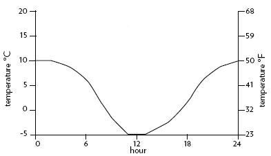
Converters: thermostat setting = 18°C discrepancy between desired and actual room temperature = maximum of (thermostat setting – room temperature ) or 0 discrepancy between inside and outside temperature = room temperature – 10°C . . . for constant outside temperature (Figures 16–18); room temperature – 24-hour outside temp . . . for full day-and night cycle (Figures 19 and 20) 24-hour outside temp ranges from 10°C (50°F) during the day to – 5°C (23°F) at night, as shown in graph
Population —for Figures 21–26
Stock: population(t) = population(t – dt) + (births – deaths ) × dt Initial stock value: population = 6.6 billion people
t = years
dt = 1 year
Run time = 100 years
Inflow: births = population × fertility
Outflow: deaths
= population
× mortality
Converters:
Figure 22:
mortality = .009 . . . or 9 deaths per 1000 population
fertility = .021 . . . or 21 births per 1000 population
Figure 23:
mortality = .030
fertility = .021
Figure 24:
mortality = .009
fertility starts at .021 and falls over time to .009 as shown in graph
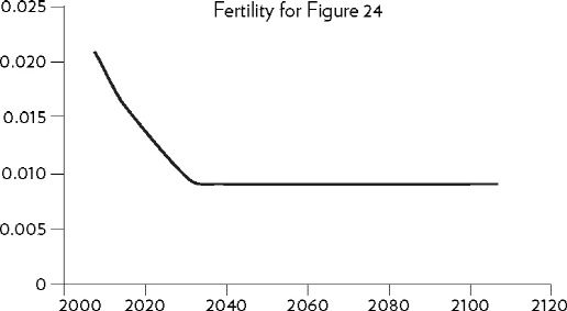
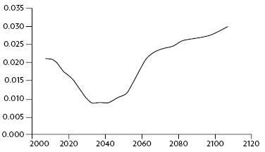
Figure 26:
mortality = .009
fertility starts at .021, drops to .009, but then rises .030 as shown in graph
Capital —for Figures 27 and 28
Stock: capital stock(t) = capital stock(t – dt) + (investment – depreciation ) × dt Initial stock value: capital stock = 100
t = years
dt = 1 year
Run time = 50 years
Inflow: investment = annual output × investment fraction
Outflow: depreciation = capital stock / capital lifetime
Converters: annual output = capital stock × output per unit capital capital lifetime = 10 years, 15 years, and 20 years . . . for three comparative model runs.
investment fraction = 20%
output per unit capital = 1/3
Business Inventory —for Figures 29–36
Stock: inventory of cars on the lot(t) = inventory of cars on the lot(t – dt) + (deliveries – sales ) × dt Initial stock values: inventory of cars on the lot = 200 cars
t = days
dt = 1 day
Run time = 100 days
Inflows: deliveries = 20 . . . for time 0 to 5; orders to factory (t – delivery delay) . . . for time 6 to 100
Outflows: sales = minimum of inventory of cars on the lot or customer demand
Converters: customer demand = 20 cars per day . . . for time 0 to 25; 22 cars per day . . . for time 26 to 100
perceived sales = sales averaged over perception delay (i.e., sales smoothed over perception delay )
desired inventory = perceived sales × 10
discrepancy = desired inventory – inventory of cars on the lot
orders to factory = maximum of (perceived sales + discrepancy ) or 0 . . . for
Figure 32; maximum of (perceived sales + discrepancy /response delay ) or 0 . . . for Figures 34–36
Delays, Figure 30:
perception delay = 0
response delay = 0
delivery delay = 0
Delays, Figure 32:
perception delay = 5 days
response delay = 3 days
delivery delay = 5 days
Delays, Figure 34:
perception delay = 2 days
response delay = 3 days
delivery delay = 5 days
Delays, Figure 35:
perception delay = 5 days
response delay = 2 days
delivery delay = 5 days
Delays, Figure 36:
perception delay = 5 days
response delay = 6 days
delivery delay = 5 days
A Renewable Stock Constrained by a Nonrenewable Resource —for Figures 37–41 Stock: resource(t) = resource(t – dt) – (extraction × dt )
Initial stock values: resource = 1000 . . . for Figures 38, 40, and 41; 1000, 2000, and 4000 . . . for three comparative model runs in Figure 39 Outflow: extraction = capital × yield per unit capital
t = years
dt = 1 year
Run time = 100 years
Stock: capital(t) = capital(t – dt) + (investment – depreciation ) × dt
Initial stock values: capital = 5 Inflow: investment = minimum of profit or growth goal
Outflow: depreciation = capital / capital lifetime
Converters: capital lifetime = 20 years
profit = (price × extraction ) – (capital × 10%) growth goal = capital × 10% . . .
for Figures 30–40; capital × 6%, 8%, 10%, and 12% . . . for four comparative model runs in Figure 40
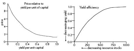
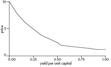
price = 3 . . . for Figures 38, 39, and 40; for Figure 41, price starts at 1.2
when yield per unit capital is high and rises to 10 as yield per unit capital falls, as shown in graph
yield per unit capital starts at 1 when resource stock is high and falls to 0 as the resource stock declines, as shown in graph
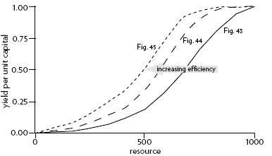
A Renewable Stock Constrained by a Renewable Resource —for Figures 42–45
Stock: resource(t) = resource(t – dt) + (regeneration – harvest ) × dt
Initial stock value: resource = 1000
Inflow: regeneration = resource × regeneration rate
Outflow: harvest = capital × yield per unit capital
t = years
dt = 1 year
Run time = 100 years
Stock: capital(t) = capital(t – dt) + (investment – depreciation ) × dt
Initial stock value: capital = 5
Inflow: investment = minimum of profit or growth goal
Outflow: depreciation = capital / capital lifetime
Converters: capital lifetime = 20
growth goal = capital × 10%
profit = (price × harvest ) – capital
price starts at 1.2 when yield per unit capital is high and rises to 10 as
yield per unit capital falls. This is the same nonlinear relationship for
price and yield as in the previous model.
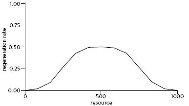
regeneration rate is 0 when the resource is either fully stocked or
completely depleted. In the middle of the resource range, regeneration rate peaks near 0.5.
yield per unit capital starts at 1 when the resource is fully stocked, but falls (non-linearly) as the resource stock declines. Yield per unit capital increases overall from least efficient in Figure 43, to slightly more efficient in Figure 44, to most efficient in Figure 45.